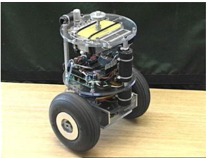
Balance car Kalman filter algorithm use experience
This time, we're discussing the use of a balance car with a Kalman filter. Let's dive into how this works based on our experience.
We use angular velocity sensors and accelerometers to measure both the angle and angular velocity. However, since the car is in motion, the angle derived from acceleration isn't entirely accurate. Additionally, due to noise interference, the readings from the angular velocity sensor are also unreliable. To address this, we need to filter these measurements using the relationship between the two sensors. That's where the Kalman filter comes in—it helps us combine these inputs to get a more accurate result.
To better understand the Kalman filter, let’s start by referencing a classic example from Baidu Encyclopedia. Before diving into the five key formulas, let’s walk through an example step by step.
Imagine we’re trying to estimate the temperature of a room. Based on our experience, we assume the temperature remains constant over time. For instance, if the current temperature is 23°C, we expect it to be roughly the same in the next minute. However, we aren’t 100% certain about this prediction—there might be some small deviations. We treat these deviations as white Gaussian noise, meaning they are random and follow a normal distribution.
In addition to our own estimation, we place a thermometer in the room. But this thermometer isn’t perfect either; its readings may differ slightly from the actual temperature. Again, we model these errors as Gaussian white noise.
Now, for each minute, we have two temperature estimates: one from our system (based on previous knowledge) and one from the thermometer. Our goal is to combine these two values along with their respective uncertainties to estimate the true temperature.
Suppose at time k, we predict the temperature to be 23°C, with a standard deviation of 5°C. The thermometer measures 25°C, with a standard deviation of 4°C. Using the Kalman gain formula:
$$ K_g = \frac{5^2}{5^2 + 4^2} = 0.78 $$
We then calculate the optimal temperature estimate as:
$$ 23 + 0.78 \times (25 - 23) = 24.56^\circ C $$
This shows that the estimated value leans more toward the thermometer reading because its uncertainty is smaller.
After obtaining the optimal estimate at time k, we update the uncertainty for the next step. The new uncertainty is calculated as:
$$ \sqrt{(1 - K_g) \times 5^2} = 2.35^\circ C $$
This process continues recursively, allowing the Kalman filter to refine its estimates over time. It only keeps track of the previous covariance, making it efficient and fast. The Kalman gain adjusts dynamically depending on the situation, which makes it highly adaptable.

Now, let's look at the code implementation. This code is adapted from online resources and is used with an AVR microcontroller:
```c
#include "Kalman.h"
float Q_angle = 0.001, Q_gyro = 0.003, R_angle = 0.5, dt = 0.005;
float P[2][2] = {
{1, 0},
{0, 1}
};
float Pdot[4] = {0, 0, 0, 0};
const char C_0 = 1;
float q_bias, angle_err, PCt_0, PCt_1, E, K_0, K_1, t_0, t_1;
void Kalman_Filter(float angle_m, float gyro_m) // gyro_m: gyro measurement
{
angle += (gyro_m - q_bias) * dt; // a priori estimate
Pdot[0] = Q_angle - P[0][1] - P[1][0]; // differential of Pk-
Pdot[1] = -P[1][1];
Pdot[2] = -P[1][1];
Pdot[3] = Q_gyro;
P[0][0] += Pdot[0] * dt; // Pk- integral
P[0][1] += Pdot[1] * dt;
P[1][0] += Pdot[2] * dt;
P[1][1] += Pdot[3] * dt;
angle_err = angle_m - angle; // zk - a priori estimate
PCt_0 = C_0 * P[0][0];
PCt_1 = C_0 * P[1][0];
E = R_angle + C_0 * PCt_0;
K_0 = PCt_0 / E;
K_1 = PCt_1 / E;
t_0 = PCt_0;
t_1 = C_0 * P[0][1];
P[0][0] -= K_0 * t_0;
P[0][1] -= K_0 * t_1;
P[1][0] -= K_1 * t_0;
P[1][1] -= K_1 * t_1;
angle += K_0 * angle_err;
q_bias += K_1 * angle_err;
angle_dot = gyro_m - q_bias;
}
```
Let’s break down what each part does.
The line `angle += (gyro_m - q_bias) * dt` represents the a priori estimate of the angle based on the gyroscope data. This uses the system's model to predict the next state.
Next, the code updates the covariance matrix `P`, which tracks the uncertainty of the system. This corresponds to the equation:
$$ P(k|k-1) = A P(k-1|k-1) A^T + Q $$
Then, the code calculates the difference between the measured angle and the predicted angle (`angle_err`) and computes the Kalman gain, which determines how much weight to give to the measurement versus the prediction.
Finally, the code updates the angle and bias using the Kalman gain, resulting in the a posteriori estimate.
Overall, this implementation is very efficient, running in under 0.5 milliseconds on a 72 MHz STM32, making it suitable for real-time applications.
thunderbolt cables,Usb4 Usb C To Type-C,Usb4 Usb-C Data Cable,Customizable Type C Thunderbolt3 Cable
Dongguan Pinji Electronic Technology Limited , https://www.iquaxusb4cable.com